Intro
Constrained optimization investigates how to minimize or maximize an objective function while satisfying one or more constraints. Instead of searching freely over the whole space, the solution must lie on the feasible set defined by the constraint, such as $C(x)=0$. The Lagrange multiplier method provides a systematic way to find candidate optima by balancing the gradient of the objective with the gradient of the constraint.
Problem definition
Let's start from a very simple constrained optimization problem:
\[ \min_x f(x) \]subject to
\[ C(x)=0. \]We can build the Lagrangian:
\[ L(x,\lambda)=f(x)-\lambda C(x). \]The solution has to satisfy the following two conditions:
\[ \frac{\partial L}{\partial \lambda}=-C(x)=0, \tag{1} \]which means the constraint has to be satisfied exactly.
And
\[ \frac{\partial L}{\partial x} = \frac{\partial f(x)}{\partial x} - \lambda \frac{\partial C(x)}{\partial x} = 0. \tag{2} \]This means that, at a regular constrained optimum, the objective has no downhill component along the feasible set. Equivalently, the gradient of the objective is balanced by the gradient of the constraint.
Why not minimize over $\lambda$?
Suppose
\[ L(x,\lambda)=f(x)-\lambda C(x). \]If the constraint is not satisfied exactly, i.e.
\[ C(x)\neq 0, \]and for a fixed $\tilde{x}$,
\[ L(\tilde{x},\lambda)=f(\tilde{x})-\lambda C(\tilde{x}). \]The value of $L$ is linearly dependent on $\lambda$, which is unbounded in the whole space. There is no minimum or maximum because we can choose $\lambda$ to make $L$ go to negative infinity or positive infinity.
Why does $\frac{\partial L}{\partial x}=0$ hold?
We know
\[ \frac{\partial L}{\partial x} = \frac{\partial f}{\partial x} - \lambda \frac{\partial C}{\partial x} = 0. \]That means
\[ \frac{\partial f}{\partial x} = \lambda \frac{\partial C}{\partial x}. \]It means:
At the constrained optimum, the gradient of the objective is balanced by the gradient of the constraint.
In physics language:
The objective wants to move $x$ downhill, but the constraint force prevents the motion.
Geometric intuition
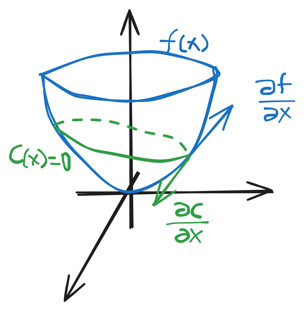 In the above figure, $f(x)$ has a global minimum, the bowl shape. The constraint is the green curve. Without the constraint,
However, the feasible set is the green curve, and the constrained minimum is the yellow point on that curve.
Why?
Notice that, at a regular point, $\nabla C$ is perpendicular to the constraint curve. If $\nabla f$ has even a small component along the curve $C(x)=0$, then we can move along $C$ to reduce the value of $f$.
Why is $\nabla C$ perpendicular to the curve?
Consider a 2D constraint:
\[ C(x,y)=0. \]Take a small movement along the curve:
\[ d\mathbf{x} = \begin{bmatrix} dx \\ dy \end{bmatrix}. \]Then
\[ C(x+dx,y+dy)=0. \]Therefore,
\[ dC=C(x+dx,y+dy)-C(x,y)=0. \]By first-order Taylor expansion,
\[ dC=\nabla C\cdot d\mathbf{x}. \]So,
\[ \nabla C\cdot d\mathbf{x}=0. \]Therefore, if $\nabla C\neq 0$, $\nabla C$ must be perpendicular to $d\mathbf{x}$, which is the tangent direction of the constraint curve.
Minimax Problem
The constrained optimization problem can also be written as
\[ \min_x \max_\lambda L(x,\lambda). \]Because
\[ \max_\lambda L(x,\lambda) = \begin{cases} f(x), & C(x)=0, \\ +\infty, & C(x)\neq 0. \end{cases} \]Then
\[ \min_x \max_\lambda L(x,\lambda) = \begin{cases} \min_x f(x), & C(x)=0, \\ \min_x +\infty, & C(x)\neq 0. \end{cases} \]Equivalently, infeasible points are punished by infinite cost, so the minimization only considers feasible points.
Example
Suppose we want to find the minimum
\[ f(x)=\frac{1}{2}x^2 \]subject to
\[ C(x)=(x-1)(x-2)=0. \]Build the Lagrangian:
\[ L(x,\lambda)=\frac{1}{2}x^2-\lambda(x-1)(x-2). \]Take the derivatives:
\[ \begin{cases} \frac{\partial L}{\partial x}=x-\lambda(2x-3), \\ \frac{\partial L}{\partial \lambda}=-(x-1)(x-2). \end{cases} \]Solve the above equations. The feasible points are
\[ x=1,\quad x=2. \]For $x=1$,
\[ 1-\lambda(2-3)=0, \]so
\[ \lambda=-1. \]For $x=2$,
\[ 2-\lambda(4-3)=0, \]so
\[ \lambda=2. \]Therefore, the Lagrange stationary points are
\[ (x,\lambda)=(1,-1),\quad (2,2). \]Since
\[ f(1)=\frac{1}{2},\qquad f(2)=2, \]therefore
\[ x=1 \]is the constrained minimum.
But wait: what is the benefit of using the Lagrange multiplier if we need to compare many feasible solutions?
Benefit of Lagrange multipliers
The benefit is: Lagrange multipliers usually reduce infinitely many feasible solutions to a much smaller set of candidate points.
Consider
\[ \min_{x,y} f(x,y)=x^2+y^2 \]subject to
\[ C(x,y)=x+y-1=0. \]The feasible solutions of the constraint are infinitely many. However, with Lagrange multipliers,
\[ L(x,y,\lambda)=x^2+y^2-\lambda(x+y-1). \]The Lagrange stationary equations are
\[ \begin{cases} \frac{\partial L}{\partial x}=2x-\lambda=0, \\ \frac{\partial L}{\partial y}=2y-\lambda=0, \\ \frac{\partial L}{\partial \lambda}=-(x+y-1)=0. \end{cases} \]From the first two equations, we know
\[ x=y=\frac{\lambda}{2}. \]Substitute it into the third one:
\[ x+y=1. \]So
\[ 2x=1. \]Therefore,
\[ x=y=\frac{1}{2}. \]We find the solution directly.
So the workflow is:
- The constraint may contain infinitely many feasible points.
- The Lagrange condition filters them down to candidate optimum points.
- Then we compare only those candidate points, not all feasible points.