This is Part I of the differentiable simulation tutorial series. In this tutorial, we introduce the basic principles of differentiable simulation using a simple yet representative FEM point-matching example. In general, two widely used approaches are the direct method and the adjoint method, which differ primarily in the order in which the required derivatives are evaluated. We derive and compare these two methods theoretically and discuss their respective computational costs. This tutorial focuses on quasi-static FEM simulation, while the next tutorial will extend the discussion to dynamic simulation.
(1) Problem statement
Consider a free-hanging 3D beam fixed on the left. It deforms under gravity. We set a target position $x_{\mathrm{target}}$ that we want a point on the beam surface, $x_{\mathrm{tracked}}$, to reach at the final equilibrium. We consider three material parameters
\[ \theta = [E,\rho,\nu], \]where $E$ is Young's modulus, $\rho$ is density, and $\nu$ is Poisson's ratio. These are the optimizable parameters.
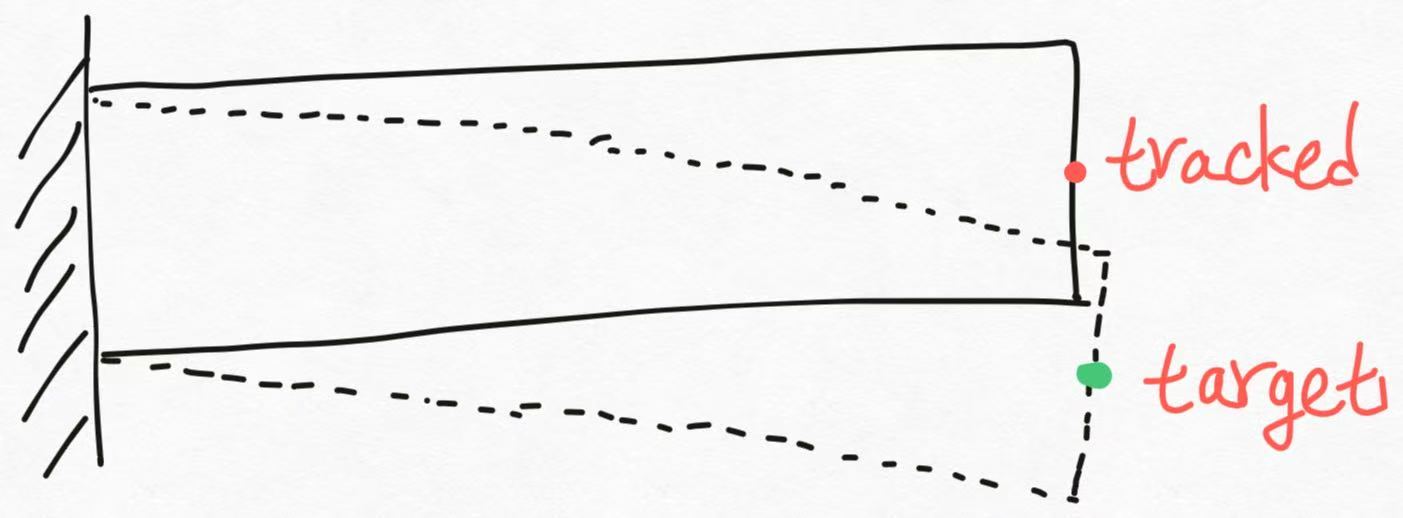 We define the loss as
where $q^*$ is the final equilibrium configuration of the simulated beam, and $s$ is a scalar scale coefficient. Our goal is to compute the derivative of loss wrt material parameters, i.e., $\frac{\partial L}{\partial \theta}$. We can then optimize $\theta$ to make tracked point reach target point using methods like gradient descent or BFGS (refer to this).
For a quasi-static FEM simulation under gravity and with no other external loads, the total potential energy is
\[ \Pi(q,\theta) = \sum_e E_e(q,E,\nu) + E_g(q,\rho), \]where $E_e(q,E,\nu)$ is the internal elastic energy of element $e$, e.g., a tetrahedron, and $E_g(q,\rho)$ is the gravitational potential energy. The dependence of $E_g$ on $\rho$ is important because density is one of the optimizable parameters.
At equilibrium, the stationarity condition is
\[ \frac{\partial \Pi}{\partial q} = R(q^*(\theta),\theta) = 0. \]Here, $R$ is the equilibrium residual, or equivalently the gradient of the total potential energy with respect to the degrees of freedom. If one defines the total physical force as $f_{\mathrm{total}}=-\partial \Pi/\partial q$, then $R=-f_{\mathrm{total}}$. Both vanish at equilibrium.
This equilibrium equation holds along the equilibrium solution $q^*(\theta)$. Taking a total derivative with respect to $\theta$ gives
\[ \frac{dR}{d\theta} = \frac{\partial R}{\partial q}\frac{dq^*}{d\theta} + \frac{\partial R}{\partial \theta} =0. \tag{1} \]We denote
\[ R_q = \frac{\partial R}{\partial q} = \frac{\partial^2 \Pi}{\partial q^2}, \]which is the Hessian of the total potential energy, i.e., the tangent stiffness matrix.
We also have
\[ R_\theta = \frac{\partial R}{\partial \theta}, \]which is the sensitivity of the equilibrium residual $R$ with respect to $\theta$, with $q$ held fixed. Because $\rho$ appears in the gravitational potential energy, the $\rho$ column of $R_\theta$ generally contains a contribution from gravity.
Rearranging Eq. (1), we obtain
\[ R_q \frac{dq^*}{d\theta} = -R_\theta. \tag{2} \]For the loss defined above, $L$ has no explicit dependence on $\theta$, so
\[ \frac{dL}{d\theta} = \left(\frac{dL}{dq}\right)^T \frac{dq^*}{d\theta}. \tag{3} \]We use the transpose because $dL/dq$ is represented here as a column vector. This equation is the starting point for both the direct method and the adjoint method. The direct method explicitly computes $dq^*/d\theta$, whereas the adjoint method avoids computing this full sensitivity matrix.
In our FEM code, there are 60 movable vertices each with 3 components. So the total number of DOFs is 180, i.e.,
\[ q \in \mathbb{R}^{180}, \qquad \theta \in \mathbb{R}^{3}. \]Therefore,
\[ R_q \in \mathbb{R}^{180\times180}, \qquad R_\theta \in \mathbb{R}^{180\times3}, \qquad \frac{dL}{dq} \in \mathbb{R}^{180\times1}, \qquad \frac{dq^*}{d\theta} \in \mathbb{R}^{180\times3}. \]$R_q$ and $R_\theta$ can be computed using automatic differentiation frameworks such as PyTorch. For automatic differentiation, Jingnan gives a very excellent introduction to it using dual value. Alternatively, they can be derived analytically using the chain rule, although this is often non-trivial. For large-scale FEM systems, explicitly forming these matrices may be expensive, and matrix-free Jacobian-vector or vector-Jacobian products can be preferable.
Obtaining the explicit expression for $dL/dq$ is relatively straightforward because the loss depends only on one tracked vertex. Therefore, the vector is largely sparse. The remaining quantity needed by the direct formulation is $dq^*/d\theta$.
(2) Direct method
The direct method first solves for $dq^*/d\theta$ from Eq. (2). Assuming $R_q$ is invertible,
\[ \frac{dq^*}{d\theta} = -R_q^{-1}R_\theta. \]Substituting this into Eq. (3) gives
\[ \frac{dL}{d\theta} = \left(\frac{dL}{dq}\right)^T (-R_q^{-1})R_\theta. \tag{4} \]Therefore, the direct method amounts to solving the linear system in Eq. (2). In this example, there are three optimizable parameters, so conceptually there are three right-hand-side solves, one for each material parameter.
In general, if there are $m$ optimizable parameters,
\[ R_q \frac{dq^*}{d\theta} = -R_\theta, \]with
\[ R_q \in \mathbb{R}^{d\times d}, \qquad \frac{dq^*}{d\theta}\in\mathbb{R}^{d\times m}, \qquad R_\theta\in\mathbb{R}^{d\times m}, \]requires $m$ right-hand-side solves with the same coefficient matrix $R_q$.
In practice, we do not explicitly compute $R_q^{-1}$. Instead, we factorize $R_q$, for example using LU, Cholesky, or $LDL^T$ when appropriate, and reuse the same factorization for all right-hand sides. Thus, the direct method requires one factorization of $R_q$ and $m$ forward/backward substitutions if a direct linear solver is used.
(3) Adjoint method
The adjoint method computes the same derivative in Eq. (4), but avoids explicitly forming
\[ R_q^{-1}R_\theta. \]Instead, it evaluates the left part first,
\[ \left(\frac{dL}{dq}\right)^T R_q^{-1}. \]Introduce the adjoint variable $\lambda$ and define it by
\[ R_q^T\lambda = L_q, \qquad \text{where } L_q = \frac{dL}{dq}. \]Conceptually,
\[ \lambda = R_q^{-T}L_q. \]Taking the transpose gives
\[ \lambda^T = L_q^T R_q^{-1} = \left(\frac{dL}{dq}\right)^T R_q^{-1}. \]Therefore,
\[ \frac{dL}{d\theta} = -\lambda^T R_\theta. \]In implementation, we solve
\[ R_q^T\lambda=L_q \]using the same kind of factorization or iterative linear solver as in the direct method. Mathematically, the adjoint variable $\lambda$ describes how the final loss responds to perturbations of the equilibrium residual. $-\lambda_i$ gives the first-order sensitivity of the loss to a perturbation of the $i_{th}$ residual equation.
For a conservative quasi-static FEM system,
\[ R_q = \frac{\partial^2\Pi}{\partial q^2} \]is symmetric, up to numerical and implementation details. Therefore,
\[ R_q^T = R_q, \]although keeping the transpose in the derivation is useful because it makes the general adjoint formulation clear.
(4) Comparison between the two methods
The direct and adjoint methods differ primarily in the order in which the products in Eq. (4) are evaluated. The direct method evaluates the expression from right to left, whereas the adjoint method effectively evaluates it from left to right.
This closely resembles forward-mode and reverse-mode automatic differentiation. For this reason, the two approaches are also commonly called the forward sensitivity method and the adjoint/reverse sensitivity method, respectively.
The evaluation order matters greatly for computational cost.
Direct method
For $d=180$ state variables and $m$ optimizable parameters,
\[ R_q \frac{dq^*}{d\theta} = -R_\theta, \]with
\[ R_q: 180\times180, \qquad \frac{dq^*}{d\theta}: 180\times m, \qquad R_\theta: 180\times m. \]This requires $m$ right-hand-side solves with the same coefficient matrix $R_q$.
Then
\[ \frac{dL}{d\theta} = \left(\frac{dL}{dq}\right)^T \frac{dq^*}{d\theta}, \]which requires one matrix multiplication:
\[ \frac{dL}{d\theta}: 1\times m, \qquad \left(\frac{dL}{dq}\right)^T: 1\times180, \qquad \frac{dq^*}{d\theta}: 180\times m. \]Adjoint method
For a single scalar loss,
\[ R_q^T\lambda = L_q, \]with
\[ R_q^T: 180\times180, \qquad \lambda: 180\times1, \qquad L_q: 180\times1. \]This requires only one right-hand-side solve.
Then
\[ \frac{dL}{d\theta} = -\lambda^T R_\theta, \]with
\[ \frac{dL}{d\theta}: 1\times m, \qquad \lambda^T: 1\times180, \qquad R_\theta: 180\times m. \]This also requires one matrix multiplication.
(5) Conclusion
Direct method and adjoint method are just applying the same chain rule to calculate required derivatives. Their calculation order determines their computational efficiency.
Suppose there are $m$ optimizable parameters and $n$ independent scalar losses. Then the direct method requires $m$ right-hand-side solves, whereas the adjoint method requires $n$ right-hand-side solves.
Therefore,
\[ \boxed{\text{Direct method: } m \text{ RHS solves}} \]and
\[ \boxed{\text{Adjoint method: } n \text{ RHS solves}}. \]A typical optimization problem has many optimizable parameters but only one scalar objective, i.e., $m\gg n$ with $n=1$. This is why the adjoint method is particularly attractive in differentiable simulation.