The Basic Problem
An integration method determines how to compute the next state from past states. Since physical properties are stored discretely on a computer, the state is also discrete. For example, we update $\mathbf{x}_{n+1}$,$\mathbf{v}_{n+1}$ from $\mathbf{x}_{n}$,$\mathbf{v}_{n}$, where $\mathbf{x}$ and $\mathbf{v}$ are position and velocity, respectively.
Most physical simulations solve an ODE system like
\[ \begin{cases} \dot{\mathbf{x}}=\mathbf{v},\\ \mathbf{M}\dot{\mathbf{v}}=\mathbf{f}(\mathbf{x},\mathbf{v},t). \end{cases} \]For conservative mechanics,
\[ \mathbf{f}(\mathbf{x},\mathbf{v},t)=-\nabla U(\mathbf{x}), \]where $U(\mathbf{x})$ is a potential energy, i.e., elastic energy due to material deformation.
The total energy of the system is the sum of kinetic energy and elastic energy:
\[ E(\mathbf{x},\mathbf{v}) = \frac{1}{2}\mathbf{v}^T\mathbf{M}\mathbf{v} + U(\mathbf{x}), \]where $\mathbf{M}$ is the mass matrix.
Now let's investigate the energy behaviour and other properties of different integration methods.
For simplicity, we consider a basic harmonic oscillator, where a unit mass ($m=1$) is attached to a spring with unit stiffness ($k=1$).
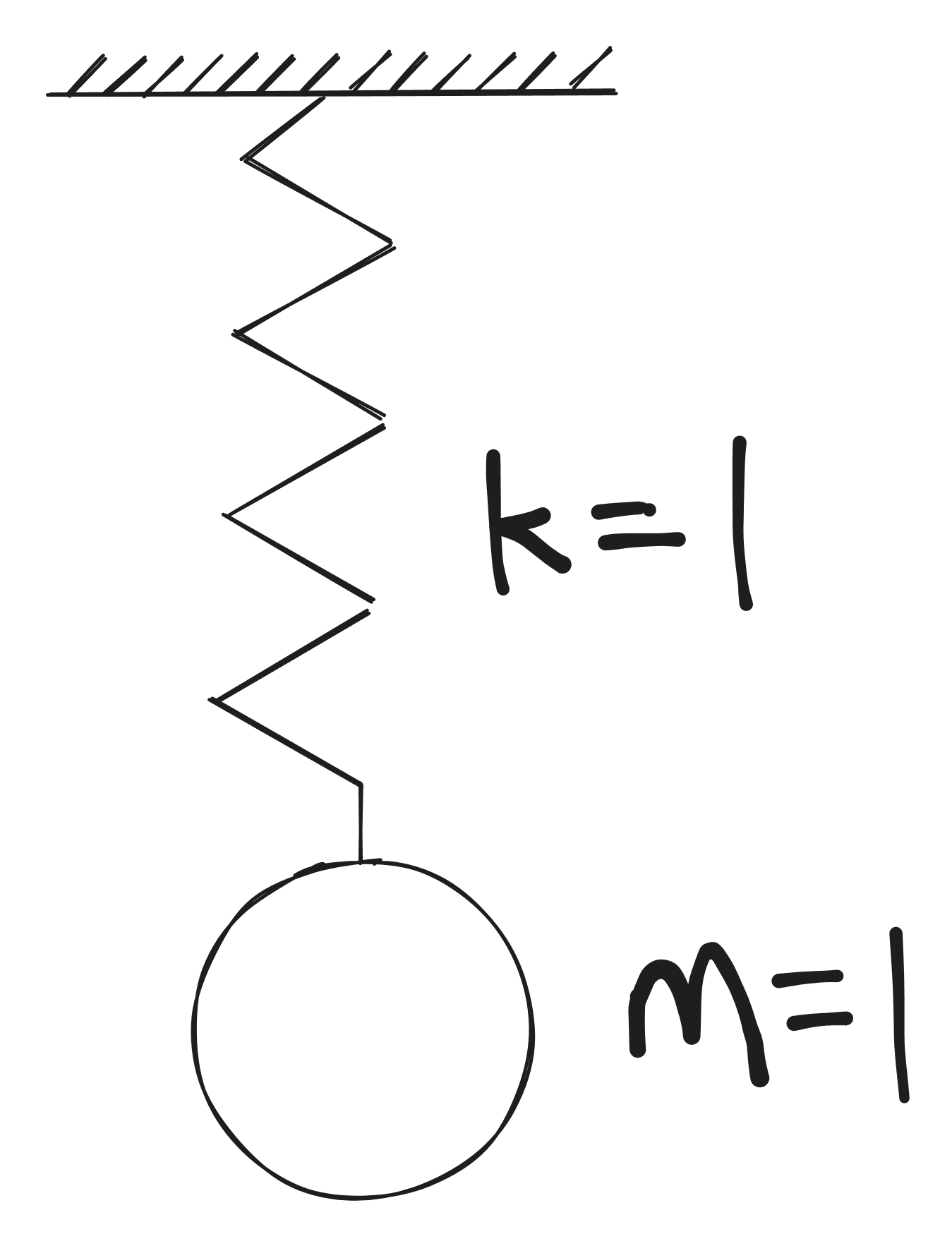
Hooke's law specifies the relationship between the spring's force and the spring's displacement. Since both the mass and stiffness are unity,
\[ \dot{\mathbf{v}}=-\mathbf{x}. \]The velocity of the unit mass is the derivative of position with respect to time:
\[ \mathbf{v}=\dot{\mathbf{x}}. \]With the initial conditions
\[ \mathbf{x}(0)=1,\qquad \mathbf{v}(0)=0, \]the exact solution is
\[ \mathbf{x}(t)=\cos(t),\qquad \mathbf{v}(t)=-\sin(t). \]The total energy of this system is
\[ E=\underbrace{\frac{1}{2}\mathbf{v}\cdot \mathbf{v}}_{\text{kinetic energy}} + \underbrace{\frac{1}{2}\mathbf{x}^2}_{\text{elastic energy}}. \]For an ideal system without damping and friction, the energy remains constant:
\[ E(t)=\frac{1}{2}. \]Forward Euler
Explicit integration calculates the future state directly from the current state, without solving any equations. Forward Euler is the simplest example:
\[ \begin{cases} \mathbf{x}_{n+1}=\mathbf{x}_n+\Delta t\,\mathbf{v}_n,\\ \mathbf{v}_{n+1}=\mathbf{v}_n+\Delta t\,\dfrac{f_n}{m} =\mathbf{v}_n-\Delta t\,\mathbf{x}_n. \end{cases} \]In matrix form,
\[ \begin{bmatrix} \mathbf{x}_{n+1}\\ \mathbf{v}_{n+1} \end{bmatrix} = \begin{bmatrix} 1 & \Delta t\\ -\Delta t & 1 \end{bmatrix} \begin{bmatrix} \mathbf{x}_n\\ \mathbf{v}_n \end{bmatrix}. \]The total energy is
\[ \begin{aligned} E_{n+1} &=\frac{1}{2}\left(\mathbf{x}_{n+1}^2+\mathbf{v}_{n+1}^2\right)\\ &=\frac{1}{2} \left[ (\mathbf{x}_n+\Delta t\,\mathbf{v}_n)^2 + (\mathbf{v}_n-\Delta t\,\mathbf{x}_n)^2 \right]\\ &=(1+\Delta t^2)\frac{1}{2}\left(\mathbf{x}_n^2+\mathbf{v}_n^2\right)\\ &=(1+\Delta t^2)E_n. \end{aligned} \]Since
\[ 1+\Delta t^2>1 \]For any nonzero timestep, the system's energy increases over time and eventually diverges.
For this undamped harmonic oscillator, Forward Euler is unstable for any nonzero timestep. This problem becomes especially severe for stiff systems, whose high-frequency modes require very small stable timesteps. The method causes an overshooting problem, which is extremely severe in stiff materials.
Backward Euler
Backward Euler belongs to the family of implicit integration methods. Implicit integration computes the current update based on the future state:
“Look at where I will be at the end of the step to decide how to move now.”
In contrast, explicit integration is:
“Look at where I am now, then move forward.”
The Backward Euler update is
\[ \begin{cases} \mathbf{x}_{n+1}=\mathbf{x}_n+\Delta t\,\mathbf{v}_{n+1},\\ \mathbf{v}_{n+1}=\mathbf{v}_n+\Delta t\,\dfrac{f_{n+1}}{m} =\mathbf{v}_n-\Delta t\,\mathbf{x}_{n+1}. \end{cases} \]Solving these two equations yields
\[ \begin{bmatrix} \mathbf{x}_{n+1}\\ \mathbf{v}_{n+1} \end{bmatrix} = \frac{1}{1+\Delta t^2} \begin{bmatrix} 1 & \Delta t\\ -\Delta t & 1 \end{bmatrix} \begin{bmatrix} \mathbf{x}_n\\ \mathbf{v}_n \end{bmatrix}. \]The total system energy is
\[ \begin{aligned} E_{n+1} &=\frac{1}{2}\left(\mathbf{x}_{n+1}^2+\mathbf{v}_{n+1}^2\right)\\ &=\frac{1}{1+\Delta t^2} \frac{1}{2}\left(\mathbf{x}_n^2+\mathbf{v}_n^2\right)\\ &=\frac{1}{1+\Delta t^2}E_n. \end{aligned} \]The energy decreases over time. Backward Euler introduces so-called numerical damping, so the system is dissipative. The larger the timestep is, the more energy is damped per timestep. For the linear harmonic oscillator, Backward Euler is stable for arbitrary timestep sizes, while introducing numerical damping.
Symplectic Euler
Symplectic Euler is also called semi-implicit Euler. As its name suggests, it is a blend of explicit and implicit integration. The velocity update is explicit, but the position update uses the updated velocity:
\[ \begin{cases} \mathbf{v}_{n+1}=\mathbf{v}_n+\Delta t\,\dfrac{f_n}{m} =\mathbf{v}_n-\Delta t\,\mathbf{x}_n,\\ \mathbf{x}_{n+1}=\mathbf{x}_n+\Delta t\,\mathbf{v}_{n+1}. \end{cases} \]Solving these equations yields
\[ \begin{bmatrix} \mathbf{x}_{n+1}\\ \mathbf{v}_{n+1} \end{bmatrix} = \begin{bmatrix} 1-\Delta t^2 & \Delta t\\ -\Delta t & 1 \end{bmatrix} \begin{bmatrix} \mathbf{x}_n\\ \mathbf{v}_n \end{bmatrix}. \]Unlike Backward Euler and Forward Euler, we cannot obtain an expression of the form
\[ E_{n+1}=kE_n. \]In fact, the original mechanical energy oscillates over time, but it remains bounded. The preserved modified energy is
\[ \widetilde{E}_{n+1} = \widetilde{E}_n = \frac{1}{2} \left( \mathbf{x}^2+\mathbf{v}^2-\Delta t\,\mathbf{x}\,\mathbf{v} \right). \]The system is stable provided that
\[ \Delta t<2. \]For a rough estimate, the modified energy and the true energy satisfy
\[ \left(1-\frac{\Delta t}{2}\right)E_n \leq \widetilde{E}_n \leq \left(1+\frac{\Delta t}{2}\right)E_n. \]Therefore, the true energy is bounded, but it oscillates.
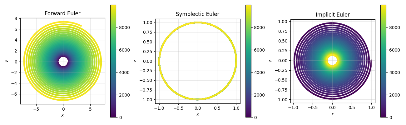
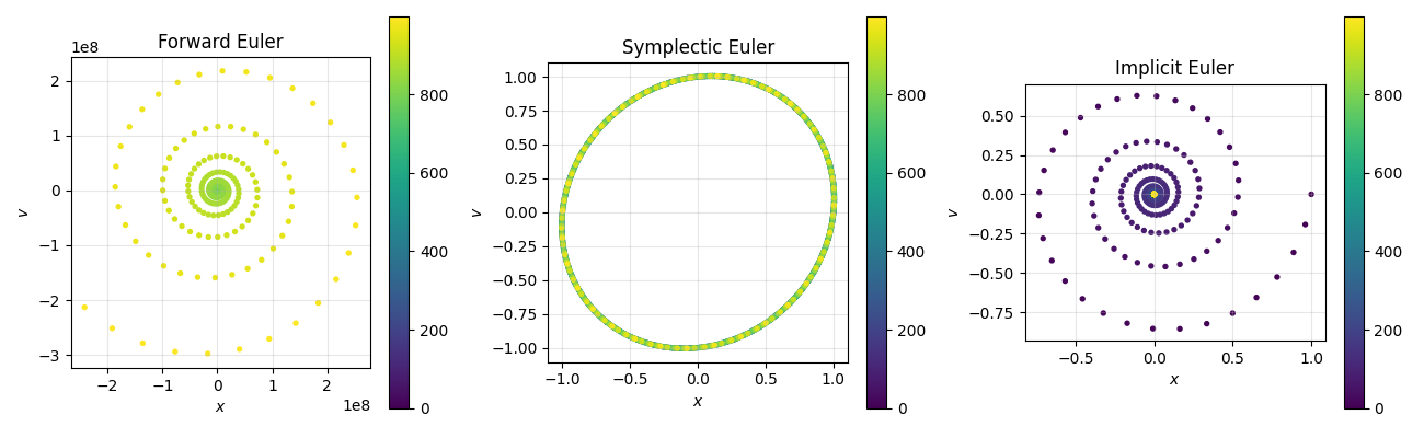
The following figures illustrate the relationship between the unit mass's position and velocity over time. Ideally, the total mechanical energy is preserved exactly without numerical damping, and the trajectory in position–velocity space is a perfect circle. However, Forward Euler produces an outward spiral, indicating artificial energy growth, while Backward Euler produces an inward spiral, indicating numerical energy dissipation. Symplectic Euler preserves energy much more effectively: its energy oscillates slightly but remains bounded. Although its position–velocity trajectory appears to be a perfect circle for a small timestep, it is actually an ellipse. This becomes apparent when a larger timestep is used, for example, $\Delta t=0.2$. The figures also show that the energy errors introduced by both Forward Euler and Backward Euler become significantly more pronounced as the timestep increases.
Verlet Integration
Verlet integration is also called Störmer--Verlet.
The Verlet integrator has good numerical stability properties. It can be classified into Position Verlet, where only position is stored explicitly, and Velocity Verlet, which stores both position and velocity. They are mathematically equivalent formulations of the same second-order symplectic method.
Position Verlet
Let's start by approximating the position at times $t+\Delta t$ and $t-\Delta t$ using Taylor expansions from time $t$:
\[ \mathbf{x}(t+\Delta t) = \mathbf{x}(t) + \Delta t\,\dot{\mathbf{x}}(t) + \frac{\Delta t^2}{2}\ddot{\mathbf{x}}(t) + \frac{\Delta t^3}{6}\mathbf{x}^{(3)}(t) + \frac{\Delta t^4}{24}\mathbf{x}^{(4)}(t) + O(\Delta t^5), \] \[ \mathbf{x}(t-\Delta t) = \mathbf{x}(t) - \Delta t\,\dot{\mathbf{x}}(t) + \frac{\Delta t^2}{2}\ddot{\mathbf{x}}(t) - \frac{\Delta t^3}{6}\mathbf{x}^{(3)}(t) + \frac{\Delta t^4}{24}\mathbf{x}^{(4)}(t) + O(\Delta t^5). \]Adding these two equations cancels out the odd derivatives:
\[ \mathbf{x}(t+\Delta t)+\mathbf{x}(t-\Delta t) = 2\mathbf{x}(t) + \Delta t^2\ddot{\mathbf{x}}(t) + O(\Delta t^4). \]Ignoring the truncation error gives
\[ \mathbf{x}_{n+1} = 2\mathbf{x}_n-\mathbf{x}_{n-1} + \Delta t^2 a_n. \]Verlet integration can be seen as using central difference to approximate the second-order derivative:
\[ a_n = \frac{ \dfrac{\mathbf{x}_{n+1}-\mathbf{x}_n}{\Delta t} - \dfrac{\mathbf{x}_n-\mathbf{x}_{n-1}}{\Delta t} }{ \Delta t }. \]Note that in the actual update, acceleration is computed directly from the force, rather than approximated by this finite difference. Verlet updates the next position directly from the previous two positions, without the need for velocity. However, velocity can be calculated using another central difference approximation:
\[ \mathbf{v}_n = \frac{\mathbf{x}_{n+1}-\mathbf{x}_{n-1}}{2\Delta t} + O(\Delta t^2), \]which is second-order accurate.
A similar half-step velocity approximation is
\[ \begin{aligned} \mathbf{v}_{n+\frac{1}{2}} &= \frac{\mathbf{x}_{n+1}-\mathbf{x}_n}{2\left(\frac{1}{2}\Delta t\right)} + O(\Delta t^2) \\ &= \frac{\mathbf{x}_{n+1}-\mathbf{x}_n}{\Delta t} + O(\Delta t^2). \end{aligned} \]This is the velocity between $n$ and $n+1$. One can also approximate velocity at $n+1$ using
\[ \mathbf{v}_{n+1} = \frac{\mathbf{x}_{n+1}-\mathbf{x}_n}{\Delta t} + O(\Delta t), \]but this is only first-order accurate.
Position Verlet is conditionally stable. It conserves a nearby discrete energy exactly:
\[ \widetilde{E}_{n+\frac{1}{2}} = \frac{1}{2} \mathbf{v}_{n+\frac{1}{2}}^2 + \frac{1}{2} \mathbf{x}_n \mathbf{x}_{n+1}. \]Velocity Verlet
Position Verlet is slightly inconvenient because velocity is not explicitly available at an integer timestep. Velocity Verlet fixes this:
\[ \mathbf{x}_{n+1} = \mathbf{x}_n + \Delta t\,\mathbf{v}_n + \frac{\Delta t^2}{2}\mathbf{a}_n, \] \[ \mathbf{v}_{n+1} = \mathbf{v}_n + \frac{\Delta t}{2} \left( \mathbf{a}_n+\mathbf{a}_{n+1} \right). \]Note that Velocity Verlet assumes that acceleration $\mathbf{a}_{n+1}$ depends only on position $\mathbf{x}$ and does not depend on velocity $\mathbf{v}_{n+1}$.
Velocity Verlet preserves a modified energy exactly:
\[ \widetilde{E}_n = \frac{1}{2} \mathbf{v}_n^2 + \frac{1}{2}(1-\frac{\Delta t^2}{4})\mathbf{x}_n^2, \]Velocity Verlet is also conditionally stable.
Leapfrog Integration
Leapfrog integration belongs to the family of Verlet methods. Its key idea is:
-
Positions are stored at integer time $n$.
-
Velocities are stored at intermediate times $n+\frac{1}{2}$.
The staggered nature makes them “leapfrog” over each other.
The update is
\[ \begin{cases} \mathbf{v}_{n+\frac{1}{2}} = \mathbf{v}_{n-\frac{1}{2}} + \Delta t\,\mathbf{a}_n, \\[4pt] \mathbf{x}_{n+1} = \mathbf{x}_n + \Delta t\,\mathbf{v}_{n+\frac{1}{2}}. \end{cases} \]Here, $\mathbf{a}_n$ is the acceleration at timestep $n$, which depends only on position $\mathbf{x}_n$.
Some key properties are:
-
Leapfrog and Position Verlet produce the same positions, provided that their initial states are initialized consistently.
-
It is second-order accurate and conditionally stable.
-
It preserves staggered energy:
Newmark Integration
Unlike Euler and Leapfrog integration, Newmark uses two parameters: $\beta$ and $\gamma$.
The update is
\[ \mathbf{x}_{n+1} = \mathbf{x}_n + \Delta t\,\mathbf{v}_n + \Delta t^2 \left[ \left(\frac{1}{2}-\beta\right)\mathbf{a}_n + \beta \mathbf{a}_{n+1} \right], \] \[ \mathbf{v}_{n+1} = \mathbf{v}_n + \Delta t \left[ (1-\gamma)\mathbf{a}_n + \gamma \mathbf{a}_{n+1} \right]. \]Note that when
\[ \beta=0, \qquad \gamma=\frac{1}{2}, \]Newmark reduces to Velocity Verlet when acceleration depends only on position.