Introduction
The variational approach is a formulation of mechanics based on energy and motion trajectories rather than directly on force. Its central idea is Hamilton's principle, which states that among all nearby possible paths connecting two configurations, the physical trajectory makes the action stationary. Unlike Newtonian mechanics, the variational approach naturally handles complex coordinates, constraints, and conservation laws. In numerical simulation, discretizing the action leads to variational integrators, which often preserve momentum and show better long-term energy behavior than methods that directly discretize force equations.
This tutorial provides a brief introduction to the variational approach. It is organized as follows. Section 2 introduces some preliminary concepts, such as variation, functionals, and conservative forces. Section 3 shows how the variational approach can be used to solve a general conservative system. Section 4 solves a simple mass-spring system using both the variational approach and Newtonian mechanics to illustrate their differences and connections. Finally, I discuss the physical meaning of Hamilton's principle.
Preliminaries
Variation and Differentiation
Variation and differentiation are two very important mathematical concepts. They both represent infinitesimal changes. However, because they look similar, they can easily cause confusion. Their physical and mathematical meanings are quite different.
Before introducing variation, let us first recall the definition of differentiation.
When the independent variable changes as
\[ x \to x + dx, \]the corresponding dependent variable changes as
\[ y \to y + dy. \]When
\[ dx \to 0, \qquad dy \to 0, \]both changes become infinitesimally small.
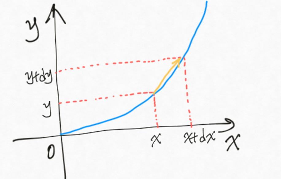
is the derivative of $y$ with respect to $x$, which gives the tangent direction of the function curve.
So, differentiation measures how a scalar or function value changes with respect to a change in its variable along the same function curve.
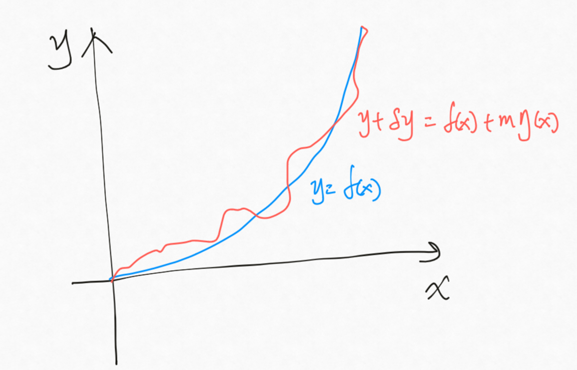
Variation, on the other hand, measures how a scalar value changes with respect to a change in a function. This scalar value is defined as a function of a function:
\[ S = \mathcal{F}[f(x)], \]where $x$ is the independent variable, $f$ is a function, $\mathcal{F}$ is a functional, and $S$ is a scalar value.
Variation is denoted by the symbol $\delta$.
For example, suppose the original function is
\[ y=f(x), \]and the perturbed function is
\[ f_\epsilon(x)=f(x)+\epsilon\eta(x), \]where $\eta(x)$ is a small perturbation of the original function.
In many cases, variation follows calculation rules similar to differentiation. For example,
\[ dy(x)=y'(x)\,dx, \] \[ \delta y(x)=y'(x)\,\delta x, \] \[ d(AB)=B\,dA+A\,dB, \] \[ \delta(AB)=B\,\delta A+A\,\delta B. \]Another commonly used symbol is the partial derivative $\partial$. It is equivalent to differentiation $d$ when a function depends only on one variable, e.g.
\[ y=f(x). \]In this case,
\[ \frac{dy(x)}{dx} = \frac{\partial y(x)}{\partial x}. \]Conventionally, people write
\[ dy(x)=y'(x)\,dx. \]However, it is not standard practice to write
\[ \partial y(x)=y'(x)\,\partial x, \]because the differential symbol must specify with respect to which variable the partial derivative is taken.
Conservative Force
A conservative force is a force whose total work is independent of the path taken. The total work depends only on the starting and ending points.
For example, the total work done by a conservative force along three trajectories, shown in blue, red, and green, is exactly the same.
Gravitational force is a typical conservative force, while frictional force is a non-conservative force.
A force $\mathbf{F}$ is conservative if there exists a scalar potential $\Phi$ such that
\[ \mathbf{F}=-\nabla \Phi. \]The Variational Approach Solves Conservative Systems
Hamilton's Principle
In physics, Hamilton's principle describes the dynamics of a physical system. A dynamical system can be formulated using a single variational scalar function called the Lagrangian. The Lagrangian contains information about the possible forces and trajectories of the physical system. The equations of motion can be obtained by taking the variation of the action, which is the time integral of the Lagrangian.
Hamilton's principle is a fundamental formulation of classical mechanics. Under suitable assumptions, it is equivalent to Newton's laws, and the Euler-Lagrange equations can be derived from it.
Mathematical Definition
Given a physical system, its generalized coordinate $\mathbf{q}$, and time $t$, where
\[ \mathbf{q}=\mathbf{q}(t), \]Hamilton's principle is
\[ \delta S[\mathbf{q}] = \delta \int_{t_0}^{t_1} L(\mathbf{q}(t),\dot{\mathbf{q}}(t),t)\,dt =0, \qquad \delta \mathbf{q}(t_0)=0, \qquad \delta \mathbf{q}(t_1)=0. \]Here, $L(\mathbf{q}(t),\dot{\mathbf{q}}(t),t)$ is called the Lagrangian function, and
\[ S[\mathbf{q}] = \int_{t_0}^{t_1} L(\mathbf{q}(t),\dot{\mathbf{q}}(t),t)\,dt \]is called the action.
Hamilton's principle says:
Among all nearby trajectories with the same starting and ending points, the physically feasible trajectory makes the action stationary.
In other words, any small perturbation near the true physical trajectory produces zero first-order change in the action $S$. That is,
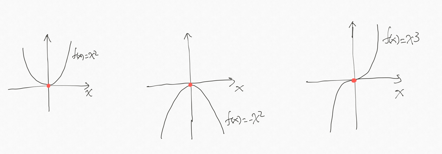
\[ \frac{\delta S}{\delta \mathbf{q}(t)}=0. \]Keep in mind that the stationary condition does not mean that the true trajectory gives the minimum value of the action. This is similar to an ordinary function $f(x)$. If
\[ f'(x)=\frac{df}{dx}=0, \]then $x$ could be a minimum point, a maximum point, or a saddle point. For example:
-
$x=0$ is a minimum point for $f(x)=x^2$.
-
$x=0$ is a maximum point for $f(x)=-x^2$.
-
$x=0$ is a saddle-like stationary point for $f(x)=x^3$.
Applying Hamilton's principle yields the Euler-Lagrange equation:
\[ \frac{d}{dt} \left( \frac{\partial L}{\partial \dot{\mathbf{q}}} \right) - \frac{\partial L}{\partial \mathbf{q}} =0. \]Building the Lagrangian
For a system consisting only of conservative forces, the process of building the Lagrangian is quite standard. Non-conservative forces need special treatment, which is outside the scope of this tutorial.
For many conservative mechanical systems with position-dependent potential energy, the Lagrangian has the standard form
\[ L=T-V. \]More general systems may require velocity-dependent potentials, constraints, or non-conservative generalized forces, which are beyond the scope of this tutorial.
Step 1: Choose the Coordinate Variables
For FEM deformable objects,
\[ \mathbf{q}=\mathbf{x}\in \mathbb{R}^{3n}. \]For a single rigid body,
\[ \mathbf{q}=(\mathbf{c},\mathbf{R}), \qquad \mathbf{R}\in SO(3). \]For an articulated rigid-body system,
\[ \mathbf{q}=(q_1,\ldots,q_m). \]Here, $q_i$ is the generalized joint coordinate, such as a hinge angle or slider displacement.
Step 2: Determine the Kinetic Energy
Here we use a deformable FEM object as an example:
\[ T= \frac{1}{2} \dot{\mathbf{q}}^T \mathbf{M} \dot{\mathbf{q}}, \]where $\mathbf{M}$ is the mass matrix.
Step 3: Find the Conservative Force Potential
Recall that any conservative force can be written as the derivative of a potential energy:
\[ \mathbf{f} = -\nabla V(\mathbf{q}). \]For example, the elastic potential is
\[ V_{\text{elastic}}(\mathbf{q}) = \sum_e V_e^0 \Psi_e(\mathbf{F}_e(\mathbf{x})). \]The gravitational potential is
\[ V_{\text{gravity}}(\mathbf{q}) = \sum_i m_i g y_i. \]In the ordinary mechanical systems considered here, the conservative potential energy is assumed to depend only on position, not velocity.
Finally, the Lagrangian is
\[ L(\mathbf{q},\dot{\mathbf{q}},t) = T(\mathbf{q},\dot{\mathbf{q}}) - V(\mathbf{q},t). \]Discrete Lagrangian
Given a mechanical system,
\[ L(\mathbf{q},\dot{\mathbf{q}}) = T(\dot{\mathbf{q}})-V(\mathbf{q}) = \frac{1}{2}\dot{\mathbf{q}}^{T}\mathbf{M}\dot{\mathbf{q}} - V(\mathbf{q}). \]The action function is
\[ S[\mathbf{q}] = \int_{t_0}^{t_1} L(\mathbf{q},\dot{\mathbf{q}})\,dt. \]The action principle states that the true motion trajectory makes the action stationary, meaning that the first variation of the action is zero:
\[ \delta S = 0. \]When $\mathbf{q}(t)$ is the true physical path, the difference between infinitesimally close neighboring paths can be considered to vanish in the first-order variation sense.
In practice, since the Lagrangian, the true path, and the action are continuous objects, we need to approximate them numerically. This usually involves two types of approximation:
-
Trajectory approximation: how to approximate the continuous position path $\mathbf{q}(t)$ using a finite number of samples, e.g. $\mathbf{q}^0,\mathbf{q}^1,\ldots$.
-
Quadrature approximation: how to approximate the time integral in the action using a finite number of samples.
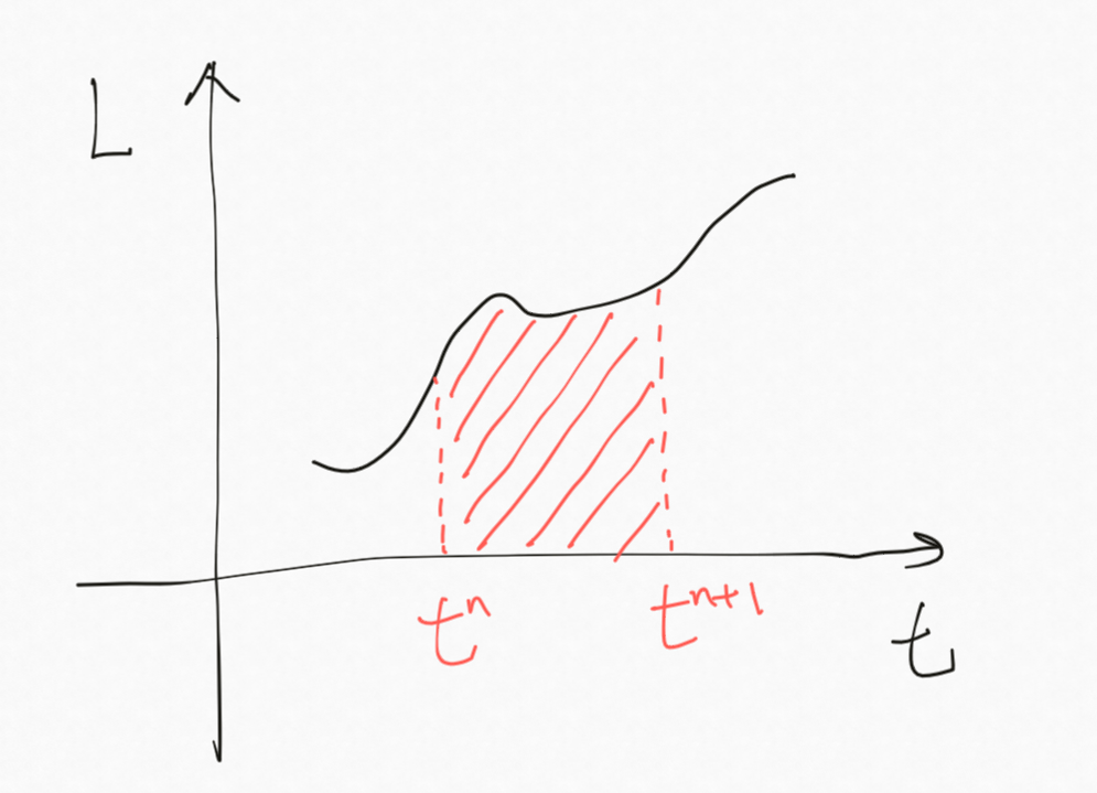
Trajectory Approximation
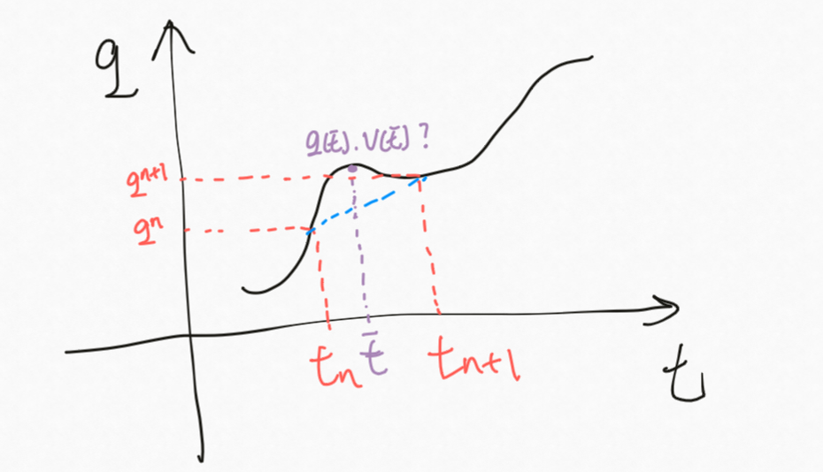
The simplest approximation is linear interpolation:
\[ \mathbf{q}(t) = \frac{t^{n+1}-t}{h}\mathbf{q}^n + \frac{t-t^n}{h}\mathbf{q}^{n+1}, \qquad h=t^{n+1}-t^n. \]The velocity is constant:
\[ \dot{\mathbf{q}}(t) = \frac{\mathbf{q}^{n+1}-\mathbf{q}^n}{h}. \]There are also higher-order approximation rules, such as quadratic, cubic, and Hermite interpolation. These can represent more complex trajectories, but they usually introduce additional internal variables.
Quadrature Approximation
This integral can be evaluated using a quadrature rule. For example, using trapezoidal quadrature,
\[ L_d(\mathbf{q}^n,\mathbf{q}^{n+1}) = \frac{h}{2} \left[ L(\mathbf{q}^n,\dot{\mathbf{q}}) + L(\mathbf{q}^{n+1},\dot{\mathbf{q}}) \right], \]where
\[ \dot{\mathbf{q}} = \frac{\mathbf{q}^{n+1}-\mathbf{q}^n}{h}. \]Substituting the mechanical Lagrangian into this formula gives
\[ \begin{aligned} L_d(\mathbf{q}^n,\mathbf{q}^{n+1}) &= \frac{h}{2} \left[ \frac{1}{2}\dot{\mathbf{q}}^T\mathbf{M}\dot{\mathbf{q}} - V(\mathbf{q}^n) \right] + \frac{h}{2} \left[ \frac{1}{2}\dot{\mathbf{q}}^T\mathbf{M}\dot{\mathbf{q}} - V(\mathbf{q}^{n+1}) \right] \\[4pt] &= \frac{1}{2h} (\mathbf{q}^{n+1}-\mathbf{q}^n)^T \mathbf{M} (\mathbf{q}^{n+1}-\mathbf{q}^n) - \frac{h}{2} \left[ V(\mathbf{q}^n)+V(\mathbf{q}^{n+1}) \right]. \end{aligned} \]This is the discrete Lagrangian under linear trajectory approximation and trapezoidal quadrature approximation.
System update
The discrete action over the entire time interval is
\[ S_d = \sum_n L_d(\mathbf{q}^n,\mathbf{q}^{n+1}). \]With fixed endpoints,
\[ \delta\mathbf{q}^0=0, \qquad \delta\mathbf{q}^N=0, \]Hamilton's principle gives
\[ \delta S_d=0 \]for all interior variations.
Since $\mathbf{q}^n$ appears in two neighboring terms,
\[ L_d(\mathbf{q}^{n-1},\mathbf{q}^n) \quad\text{and}\quad L_d(\mathbf{q}^n,\mathbf{q}^{n+1}), \]we get the discrete Euler-Lagrange equation:
\[ D_2L_d(\mathbf{q}^{n-1},\mathbf{q}^n) + D_1L_d(\mathbf{q}^n,\mathbf{q}^{n+1}) = 0. \]Here, $D_1$ and $D_2$ denote derivatives with respect to the first and second arguments.
For the discrete Lagrangian above,
\[ D_2L_d(\mathbf{q}^{n-1},\mathbf{q}^n) = \frac{1}{h} \mathbf{M}(\mathbf{q}^n-\mathbf{q}^{n-1}) - \frac{h}{2} \nabla V(\mathbf{q}^n), \]and
\[ D_1L_d(\mathbf{q}^n,\mathbf{q}^{n+1}) = -\frac{1}{h} \mathbf{M}(\mathbf{q}^{n+1}-\mathbf{q}^n) - \frac{h}{2} \nabla V(\mathbf{q}^n). \]Substituting them into the discrete Euler-Lagrange equation gives
\[ -\frac{1}{h}\mathbf{M}(\mathbf{q}^{n+1}-\mathbf{q}^n) + \frac{1}{h}\mathbf{M}(\mathbf{q}^n-\mathbf{q}^{n-1}) - h\nabla V(\mathbf{q}^n) = 0. \]Rearranging,
\[ \mathbf{M} \frac{\mathbf{q}^{n+1}-2\mathbf{q}^n+\mathbf{q}^{n-1}}{h^2} + \nabla V(\mathbf{q}^n) = 0. \]This equation is equivalent to the Störmer-Verlet integrator.
The whole route can be summarized as:
\[ \boxed{ \mathbf{q}(t) \to \text{choose } \mathbf{q}^n \to \text{choose } L_{d} \to \delta S_d=0 \to \text{discrete Euler--Lagrange equation} \to \text{time integrator rule} } \]Using different combinations of trajectory approximation and quadrature approximation leads to various time integration rules. Here is a brief summary of these time integrators.
| Trajectory approximation | Quadrature approximation | Discrete Lagrangian | Time integration rule |
|---|---|---|---|
| Linear | Left endpoint | $L_d=hL(\mathbf{q}^n,\mathbf{v}^{n,n+1})$ | Symplectic Euler A |
| Linear | Right endpoint | $L_d=hL(\mathbf{q}^{n+1},\mathbf{v}^{n,n+1})$ | Symplectic Euler B |
| Linear | Trapezoidal endpoint | $L_d=\dfrac{h}{2}\left[L(\mathbf{q}^n,\mathbf{v}^{n,n+1})+L(\mathbf{q}^{n+1},\mathbf{v}^{n,n+1})\right]$ | Störmer-Verlet style |
| Subdivided step with midpoint state | Gauss midpoint | Uses internal midpoint stages | Implicit midpoint Gauss variational integrator |
| Cubic or higher polynomial | Gauss-Legendre | Multiple internal stages | Higher-order implicit variational integrator |
Basically, first-order trajectories plus low-order quadrature lead to simple, cheap rules like symplectic Euler. Higher-order trajectories or higher-order quadrature lead to higher-order variational time integrators.
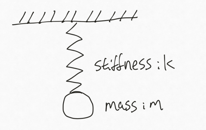
A Concrete Example
Here we use the classical mass-spring system to show the difference between the variational approach and Newtonian mechanics.
Variational Approach
The kinetic energy and elastic potential energy are defined as follows. Let $x$ denote the displacement from the spring's rest length, and ignore gravity. Equivalently, for a vertical spring under gravity, let $x$ denote the displacement from the static equilibrium position. Then
\[ \begin{cases} T(\dot{x})=\dfrac{1}{2}m\dot{x}^2,\\[4pt] V(x)=\dfrac{1}{2}kx^2. \end{cases} \]The Lagrangian is
\[ L(x,\dot{x})=T-V =\dfrac{1}{2}m\dot{x}^2-\dfrac{1}{2}kx^2. \]The action is
\[ S[x]=\int_{t_0}^{t_1} \left( \dfrac{1}{2}m\dot{x}^2-\dfrac{1}{2}kx^2 \right)\,dt. \]Let $t_n=nh$, and $x^n=x(t_n)$.
Using linear interpolation for trajectory approximation and trapezoidal integration for quadrature approximation,
\[ L_d(x^n,x^{n+1}) = \dfrac{m}{2h}(x^{n+1}-x^n)^2 - \dfrac{kh}{4} \left[ (x^n)^2+(x^{n+1})^2 \right]. \]The discrete action is
\[ S_d=\sum_n L_d(x^n,x^{n+1}). \]According to Hamilton's principle,
\[ \delta S_d=0. \]We get
\[ \left[ \dfrac{m}{h}(x^n-x^{n-1}) - \dfrac{hk}{2}x^n \right] + \left[ -\dfrac{m}{h}(x^{n+1}-x^n) - \dfrac{hk}{2}x^n \right] =0. \]Rearranging,
\[ m\dfrac{x^{n+1}-2x^n+x^{n-1}}{h^2} + kx^n =0. \tag{1} \]Therefore, we get the Störmer-Verlet position update rule:
\[ x^{n+1} = 2x^n-x^{n-1} - \dfrac{kh^2}{m}x^n. \]Newtonian Mechanics
Newton's second law says
\[ m\ddot{x}=f. \]For a spring, Hooke's law states
\[ f=-kx. \]Therefore, the force balance of the system is
\[ m\ddot{x}+kx=0. \]Let's approximate the acceleration by central difference:
\[ \ddot{x}(t_n) \approx \dfrac{ \dfrac{x^{n+1}-x^n}{h} - \dfrac{x^n-x^{n-1}}{h} }{h} = \dfrac{x^{n+1}-2x^n+x^{n-1}}{h^2}. \]Substituting this into the equation of motion gives
\[ m\dfrac{x^{n+1}-2x^n+x^{n-1}}{h^2} + kx^n =0. \tag{2} \]Comparison
In this particular example, with this choice of discrete Lagrangian and central-difference acceleration, Eq. (1) and Eq. (2) are exactly the same. Therefore, the two derivations lead to the same update rule, although their logic is different.
Newtonian route:
\[ \boxed{ \text{Force balance } \to m\ddot{\mathbf{x}}=\mathbf{f} \to \text{approximate } \ddot{\mathbf{x}} \to \text{update rule} } \]Variational route:
\[ \boxed{ \text{Action } \to \text{Lagrangian } \mathbf{L=T-V} \to \text{discrete Lagrangian } \mathbf{L}_{d} \to \text{Hamilton's principle } \delta S_d=0 \to \text{update rule } } \]Physical and Mathematical Meaning of Hamilton's Principle
Hamilton's principle is a fundamental rule for conservative mechanical systems. Under suitable assumptions, it can be shown to be equivalent to Newton's second law. The following discussion gives an intuition for the principle. It is not a strict mathematical proof.
Consider an elastic deformable body. For now, ignore damping and non-conservative forces. Let
\[ L(\mathbf{x},\dot{\mathbf{x}}) = \frac{1}{2}\dot{\mathbf{x}}^{T}\mathbf{M}\dot{\mathbf{x}} - \psi(\mathbf{x}). \]The action is
\[ S[\mathbf{x}] = \int_{t_0}^{t_1} \left[ \frac{1}{2}\dot{\mathbf{x}}^{T}\mathbf{M}\dot{\mathbf{x}} - \psi(\mathbf{x}) \right]dt. \]Now perturb the path slightly using a small $\epsilon$:
\[ \mathbf{x}(\epsilon,t) = \mathbf{x}(t)+\epsilon\boldsymbol{\eta}(t), \] \[ \dot{\mathbf{x}}(\epsilon,t) = \dot{\mathbf{x}}(t)+\epsilon\dot{\boldsymbol{\eta}}(t). \]The perturbed action is
\[ S[\mathbf{x}(\epsilon,t)] = \int_{t_0}^{t_1} \left[ \frac{1}{2} \left( \dot{\mathbf{x}}+\epsilon\dot{\boldsymbol{\eta}} \right)^T \mathbf{M} \left( \dot{\mathbf{x}}+\epsilon\dot{\boldsymbol{\eta}} \right) - \psi \left( \mathbf{x}+\epsilon\boldsymbol{\eta} \right) \right]dt. \]Differentiate with respect to $\epsilon$ and evaluate at $\epsilon=0$:
\[ \delta S = \left. \frac{d}{d\epsilon} S[\mathbf{x}(\epsilon,t)] \right|_{\epsilon=0}. \]Therefore,
\[ \delta S = \int_{t_0}^{t_1} \left[ \dot{\boldsymbol{\eta}}^T \mathbf{M} \dot{\mathbf{x}} - \boldsymbol{\eta}^T \nabla \psi(\mathbf{x}) \right]dt. \]Assume $\mathbf{M}$ is constant, as in standard nodal coordinates for many FEM systems. Then
\[ \frac{d}{dt}(\mathbf{M}\dot{\mathbf{x}}) = \mathbf{M}\ddot{\mathbf{x}}. \]Integrate the first term by parts:
\[ \int_{t_0}^{t_1} \dot{\boldsymbol{\eta}}^T \mathbf{M} \dot{\mathbf{x}}\,dt = \left[ \boldsymbol{\eta}^T \mathbf{M} \dot{\mathbf{x}} \right]_{t_0}^{t_1} - \int_{t_0}^{t_1} \boldsymbol{\eta}^T \mathbf{M} \ddot{\mathbf{x}}\,dt. \]Because the variations of the starting and ending points are zero,
\[ \boldsymbol{\eta}(t_0) = \boldsymbol{\eta}(t_1) = 0. \]Therefore,
\[ \left[ \boldsymbol{\eta}^T \mathbf{M} \dot{\mathbf{x}} \right]_{t_0}^{t_1} = 0. \]Thus,
\[ \delta S = - \int_{t_0}^{t_1} \boldsymbol{\eta}^T \left[ \mathbf{M}\ddot{\mathbf{x}} + \nabla\psi(\mathbf{x}) \right]dt. \]Here,
\[ \mathbf{M}\ddot{\mathbf{x}} + \nabla\psi(\mathbf{x}) \]is the residual.
Hamilton's principle requires
\[ \delta S=0 \]for every possible perturbation function $\boldsymbol{\eta}(t)$.
Since $\boldsymbol{\eta}(t)$ is arbitrary, the only way for this integral to vanish for every perturbation is
\[ \mathbf{M}\ddot{\mathbf{x}} + \nabla\psi(\mathbf{x}) = 0. \]We know
\[ \mathbf{f}_{\mathrm{int}} = -\nabla\psi(\mathbf{x}). \]Thus, for the elastic system considered here with no external forces,
\[ \mathbf{M}\ddot{\mathbf{x}} = \mathbf{f}_{\mathrm{int}}. \]